Project 2a: Image Compression

Overview

Implement lossy image compression using principal component extraction (wiki, slides), where a greyscale image is partitioned into non-overlapping fixed-size rectangular blocks, which are then encoded using only the first few principal components. Use the APEX algorithm (slides p. 15; Diamantaras et al. 1994) to train the network.

Deadline: April 25th, 2019

Method

1. load and partition image:
   • generally: for some block size \(w \times h\), partition the input image (of size \(W \times H\))
     into \((W/w) \cdot (H/h)\) non-overlapping rectangular blocks
     • JPEG compression uses a fixed 8x8 block size; do so as well
2. find the first \(1 \leq k \leq w \cdot h\) principal components (use \(k \geq 8\)):
   • flatten the \(w \times h\) blocks to vectors in \(wh\)-dimensional space
   • find the first principal component using¹ Oja’s rule for the first neuron
   • train the remaining neurons sequentially:²
     • for \(i \in 2 \ldots k\) find the \(i\)-th principal component using the APEX algotithm
       • \(1..i-1\)-th neurons are already trained (cf. mathematical induction)
       • iteratively train the \(i\)-th neuron:
         • lateral weights should converge to zeroes
         • forward weights will then have converged to the \(i\)-th PC
3. encode image:
   • for each image block, output only the coefficients for the first \(k\) components
     • unless \(k = w \cdot h\), this encoding is lossy
   • in a practical algorithm, the next stage would be output into a file,
     using some sort of entropy coding (usually Arithmetic/Range or Huffman)
4. reconstruct image:
   • using only the principal component vectors and coefficients from the previous step

Hints

• use small initial weights, consider keeping their mean zero
• use a small learning rate; a decreasing schedule (as in training SOMs) might also help
• as in Oja’s and GHA algorithms:
  • vectors representing different neurons should converge to be perpendicular
  • the length of such vectors should converge to one (cf. stabilizing term/normalization)
• principal components are unique (disregarding sign and limited by numerical accuracy)
  • consider implementing another method (GHA, SVD) to compare the results

Report

Using this greyscale 256x256 image of Elaine:

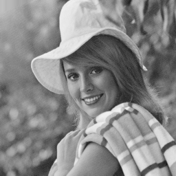
• show the result of compression for at least three different values of \(k\)
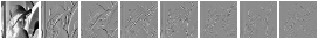
• visualize the eight most significant extracted components (as 2D images)
• plot the eigenvalues of the PCA correlation matrix in decreasing order
• examine, how well do the principal components generalize between images
  1. find two images (e.g. close portraits) similar to the sample
     • rescale if sizes differ
  2. extract principal components from the sample
  3. use them to encode and reconstruct the two images

Bonus

Implement a second way of finding the principal components, using an autoassociative network (autoencoder, wiki) with one linear hidden layer and output layer.

Try using:

1. two separate weight matrices:
   • \(\mathbf{W}^{hid}\) for input-to-hidden
   • \(\mathbf{W}^{out}\) for hidden-to-output
2. one shared weight matrix:
   • \(\mathbf{W}_{hid} = \mathbf{W}\)
   • \(\mathbf{W}_{out} = \mathbf{W}^T\)

Compare the results of the MLP variants with Oja/GHA/APEX algorithms, both qualitatively and quantitatively.

Example

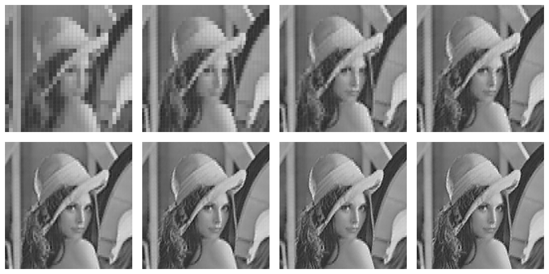
The first eight principal components of 8x8 blocks from a 256x256 image of Lenna:

The 32x32 coefficients for the components:

The reconstructions from the first one, first two, … first eight components:

---

1. First neurons learn in the exact same way in Oja’s, GHA and APEX algorithms.↩

2. Neurons in GHA can also be trained in this manner, but also converge when trained simultaneously. APEX is decidedly more fussy.↩